Design of Chebyshev Filters
This article explains the design procedure for Chebyshev filters. It shows how to determine the filter order from a specification, compute the poles, and find the coefficients of the second-order sections. A Python (SciPy) implementation example is also included.
Design specification
Designing a Chebyshev Type I low-pass filter requires the following four parameters:
- $\omega_p$: passband edge frequency (cutoff frequency)
- $\omega_s$: stopband edge frequency
- $R_p$: passband ripple [dB] (maximum attenuation within the passband)
- $A_s$: stopband attenuation [dB] (minimum attenuation within the stopband)
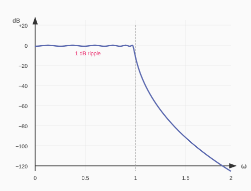
On normalization: In the design calculations the passband edge frequency is normalized to $\omega_p = 1$ rad/s. At the end, frequency scaling converts it back to the actual frequency.
Order-determination formula
Order formula for Chebyshev Type I
The minimum order $n$ that meets a given specification can be computed from the following formula:
\begin{equation} n \geq \dfrac{\cosh^{-1}\left(\sqrt{\dfrac{10^{A_s/10} - 1}{10^{R_p/10} - 1}}\right)}{\cosh^{-1}(\omega_s / \omega_p)} \label{eq:order} \end{equation}Comparison with Butterworth
For reference, the order formula for a Butterworth filter is:
\begin{equation} n_{\text{Butterworth}} \geq \dfrac{\log\left(\sqrt{\dfrac{10^{A_s/10} - 1}{10^{R_p/10} - 1}}\right)}{\log(\omega_s / \omega_p)} \label{eq:order-butter} \end{equation}In the Chebyshev formula the $\log$ is replaced by $\cosh^{-1}$. Since $\cosh^{-1}(x) \approx \log(2x)$ the numerators are nearly equal, but the denominator changes from $\log(\omega_s/\omega_p)$ to $\cosh^{-1}(\omega_s/\omega_p)$, so Chebyshev meets the same specification at a lower order (the exact reduction depends on the specification).
Numerical example
Specification: $R_p = 1$ dB, $A_s = 40$ dB, $\omega_s/\omega_p = 2$
$$ \varepsilon = \sqrt{10^{0.1} - 1} \approx 0.5088 $$ $$ \sqrt{\dfrac{10^{4} - 1}{10^{0.1} - 1}} = \sqrt{\dfrac{9999}{0.2589}} \approx 196.5 $$ $$ n \geq \dfrac{\cosh^{-1}(196.5)}{\cosh^{-1}(2)} = \dfrac{5.98}{1.32} \approx 4.5 $$Therefore $n = 5$ is required. For the same specification a Butterworth filter would need $n = 8$, so Chebyshev achieves it at a lower order.
Design procedure
Step 1: Determine the order and the ripple parameter
Compute the order $n$ from Eq. \eqref{eq:order} (rounding up) and find the ripple parameter:
$$\varepsilon = \sqrt{10^{R_p/10} - 1}$$Step 2: Compute the ellipse parameters
Compute the parameters of the ellipse on which the poles are distributed:
$$\eta = \dfrac{1}{n}\sinh^{-1}\left(\dfrac{1}{\varepsilon}\right)$$Semi-axes of the ellipse:
$$a = \sinh(\eta), \quad b = \cosh(\eta)$$Step 3: Compute the poles
For $m = 0, 1, \ldots, n-1$:
$$x_m = \dfrac{(2m+1)\pi}{2n}$$ $$p_m = -\sin(x_m) \cdot a + j\cos(x_m) \cdot b$$(Use only the left-half-plane poles.)
Step 4: Factor into second-order sections
Combine complex-conjugate pairs to build second-order sections:
$$H_k(s) = \dfrac{\omega_{0,k}^2}{s^2 + \dfrac{\omega_{0,k}}{Q_k}s + \omega_{0,k}^2}$$where:
$$\omega_{0,k} = |p_k|, \quad Q_k = \dfrac{|p_k|}{-2\text{Re}(p_k)}$$Step 5: Frequency scaling
From the normalized filter ($\omega_p = 1$) to the actual cutoff frequency $\omega_c$:
$$s \to \dfrac{s}{\omega_c}$$Multiply every $\omega_0$ by $\omega_c$.
Step 6: Gain adjustment
For even orders, adjust the DC gain to be $-R_p$ dB:
$$K = \dfrac{1}{\sqrt{1 + \varepsilon^2}}$$For odd orders, the DC gain is 0 dB, so $K = 1$.
Design example
Let us design a normalized Chebyshev Type I low-pass filter with a passband ripple of 1 dB and order $n = 6$.
Computing the parameters
$$ \varepsilon = \sqrt{10^{0.1} - 1} \approx 0.5088 $$ $$ \eta = \dfrac{1}{6}\sinh^{-1}\left(\dfrac{1}{0.5088}\right) \approx 0.2384 $$ $$ a = \sinh(0.2384) \approx 0.2406, \quad b = \cosh(0.2384) \approx 1.0287 $$Pole locations
| $m$ | $x_m$ | Pole $p_m$ | $\omega_0$ | $Q$ |
|---|---|---|---|---|
| 0 | $\pi/12 = 15°$ | $-0.0623 + j0.9935$ | 0.9955 | 7.99 |
| 1 | $3\pi/12 = 45°$ | $-0.1701 + j0.7275$ | 0.7471 | 2.20 |
| 2 | $5\pi/12 = 75°$ | $-0.2324 + j0.2662$ | 0.3534 | 0.76 |
(Left-half-plane poles only. $m = 3, 4, 5$ are conjugate poles and are omitted.)
Coefficients of the second-order sections
| Section | $\omega_0$ | $Q$ | Denominator polynomial |
|---|---|---|---|
| 1 | 0.9955 | 7.99 | $s^2 + 0.1246s + 0.9910$ |
| 2 | 0.7471 | 2.20 | $s^2 + 0.3398s + 0.5582$ |
| 3 | 0.3534 | 0.76 | $s^2 + 0.4649s + 0.1249$ |
Cascade order: When cascading the sections, place the section with the lowest $Q$ (Section 3) at the input and the section with the highest $Q$ (Section 1) at the output. This optimizes the dynamic range and the noise behavior.
Python implementation
Design with SciPy
import numpy as np
from scipy.signal import cheby1, cheby1ord, freqs, tf2zpk

# Specification
Rp = 1.0    # passband ripple [dB]
As = 40.0   # stopband attenuation [dB]
wp = 1.0    # passband edge frequency [rad/s]
ws = 2.0    # stopband edge frequency [rad/s]

# Order determination
n, Wn = cheby1ord(wp, ws, Rp, As, analog=True)
print(f"Required order: {n}")
print(f"Cutoff frequency: {Wn:.4f} rad/s")

# Filter design
b, a = cheby1(n, Rp, Wn, btype='low', analog=True)
print(f"\nNumerator coefficients b: {b}")
print(f"Denominator coefficients a: {a}")

# Zero-pole-gain form
z, p, k = tf2zpk(b, a)
print(f"\nPoles:")
for i, pole in enumerate(p):
    print(f"  p{i}: {pole:.4f}, |p|={np.abs(pole):.4f}, Q={np.abs(pole)/(-2*pole.real):.2f}")
Converting poles to second-order sections
from scipy.signal import zpk2sos

# Convert to second-order-section form
sos = zpk2sos(z, p, k)

print("Second-order sections (sos):")
print("  [b0, b1, b2, a0, a1, a2]")
for i, section in enumerate(sos):
    print(f"  Section {i+1}: {section}")

# Convert to standard-form parameters
print("\nStandard-form parameters:")
for i, section in enumerate(sos):
    b0, b1, b2, a0, a1, a2 = section
    omega0 = np.sqrt(a2/a0)
    Q = omega0 / (a1/a0)
    print(f"  Section {i+1}: ω₀ = {omega0:.4f}, Q = {Q:.4f}")
Plotting the frequency response
import matplotlib.pyplot as plt

# Frequency response
w = np.logspace(-1, 1, 500)
w, H = freqs(b, a, w)

fig, (ax1, ax2) = plt.subplots(2, 1, figsize=(10, 8))

# Magnitude response
ax1.semilogx(w, 20*np.log10(np.abs(H)))
ax1.axhline(-Rp, color='r', linestyle='--', label=f'Passband ripple ({-Rp} dB)')
ax1.axhline(-As, color='g', linestyle='--', label=f'Stopband attenuation ({-As} dB)')
ax1.axvline(wp, color='b', linestyle=':', alpha=0.5)
ax1.axvline(ws, color='b', linestyle=':', alpha=0.5)
ax1.set_ylabel('Magnitude [dB]')
ax1.set_ylim(-60, 5)
ax1.legend()
ax1.grid(True)

# Phase response
ax2.semilogx(w, np.unwrap(np.angle(H)) * 180/np.pi)
ax2.set_xlabel('Frequency [rad/s]')
ax2.set_ylabel('Phase [degrees]')
ax2.grid(True)

plt.tight_layout()
plt.show()
Component-value calculation (for Sallen-Key)
def sallen_key_components(omega0, Q, R):
    """
    Compute the component values of a Sallen-Key circuit (R1=R2=R)

    Parameters:
        omega0: natural angular frequency [rad/s]
        Q: Q factor
        R: resistance [Ω]

    Returns:
        C1, C2: capacitor values [F]
    """
    C2 = 1 / (2 * Q * omega0 * R)
    C1 = 2 * Q / (omega0 * R)
    return C1, C2

# Design example: 1 kHz cutoff, R = 10 kΩ
fc = 1000  # Hz
R = 10000  # Ω
omega_scale = 2 * np.pi * fc

print(f"Cutoff frequency: {fc} Hz")
print(f"Resistance: {R/1000} kΩ")
print()

for i, section in enumerate(sos):
    b0, b1, b2, a0, a1, a2 = section
    omega0_norm = np.sqrt(a2/a0)
    Q = omega0_norm / (a1/a0)
    omega0_actual = omega0_norm * omega_scale

    C1, C2 = sallen_key_components(omega0_actual, Q, R)

    print(f"Section {i+1}:")
    print(f"  ω₀ = {omega0_actual:.1f} rad/s ({omega0_actual/2/np.pi:.1f} Hz)")
    print(f"  Q = {Q:.3f}")
    print(f"  C₁ = {C1*1e9:.2f} nF")
    print(f"  C₂ = {C2*1e9:.2f} nF")
    print()
Designing a Type II filter
Designing a Chebyshev Type II (inverse Chebyshev) filter follows a similar procedure, but the parameters you specify are different.
Order-determination formula (Type II)
The Chebyshev order formula is common to Type I and Type II and involves both the passband ripple $R_p$ and the stopband attenuation $A_s$ (identical to Eq.\eqref{eq:order}):
\begin{equation} n \geq \dfrac{\cosh^{-1}\left(\sqrt{\dfrac{10^{A_s/10} - 1}{10^{R_p/10} - 1}}\right)}{\cosh^{-1}(\omega_s / \omega_p)} \label{eq:order-type2} \end{equation}Because the Type II passband is monotonic (maximally flat), $R_p$ is given as the allowed deviation at the passband edge. The Python example below uses 3 dB for the passband specification.
Python implementation (Type II)
from scipy.signal import cheby2, cheby2ord

# Specification
As = 40.0   # stopband attenuation [dB]
wp = 1.0    # passband edge frequency [rad/s]
ws = 2.0    # stopband edge frequency [rad/s]

# Order determination
n, Wn = cheby2ord(wp, ws, 3, As, analog=True)  # 3 dB is the passband
print(f"Required order: {n}")

# Filter design
b, a = cheby2(n, As, Wn, btype='low', analog=True)

# Frequency response
w = np.logspace(-1, 1, 500)
w, H = freqs(b, a, w)

plt.figure(figsize=(10, 4))
plt.semilogx(w, 20*np.log10(np.abs(H)))
plt.axhline(-As, color='r', linestyle='--', label=f'Stopband ({-As} dB)')
plt.xlabel('Frequency [rad/s]')
plt.ylabel('Magnitude [dB]')
plt.title('Chebyshev Type II Filter')
plt.legend()
plt.grid(True)
plt.ylim(-60, 5)
plt.show()
Notes on Type II: Because Type II has zeros on the imaginary axis, its implementation as an analog circuit is more complex than Type I. Realizing the zeros requires biquad circuits or state-variable filters. See the circuit article.
Frequency transformations
Transformations from a normalized low-pass filter to other filter types:
| Transformation | Substitution | Description |
|---|---|---|
| LP → LP | $s \to s/\omega_c$ | Frequency scaling |
| LP → HP | $s \to \omega_c/s$ | Convert to high-pass |
| LP → BP | $s \to \dfrac{s^2 + \omega_0^2}{Bs}$ | Convert to band-pass ($B$ is the bandwidth) |
| LP → BS | $s \to \dfrac{Bs}{s^2 + \omega_0^2}$ | Convert to band-stop |
Key parameters for band-pass / band-stop design
When designing a band-pass filter (BPF) or a band-stop filter (BEF / notch), it is important to understand the following parameters.
Center frequency and bandwidth
- Center frequency $f_0$ (or $\omega_0$)
- The frequency at the center of the passband (BPF) or the stopband (BEF). A BPF has its maximum gain at this frequency; a BEF has its maximum attenuation there.
- Bandwidth $B$ (or $\Delta\omega$)
- The width of the passband for a BPF, or of the stopband for a BEF. It is defined as the difference between the upper frequency $f_H$ and the lower frequency $f_L$ at the ripple level. \begin{equation} B = f_H - f_L \end{equation}
Geometric-mean center frequency
In filter theory the center frequency is often defined as the geometric mean of the upper and lower frequencies:
\begin{equation} f_0 = \sqrt{f_L \cdot f_H} \end{equation}This means that on a logarithmic frequency axis $f_0$ sits exactly halfway between $f_L$ and $f_H$. Note that it differs from the arithmetic mean $(f_L + f_H)/2$.
Fractional bandwidth and Q factor
The fractional bandwidth, which is the bandwidth normalized by the center frequency, and its reciprocal the Q factor, are important measures of how "narrow" a BPF/BEF is.
\begin{equation} \text{Fractional bandwidth} = \dfrac{B}{f_0}, \quad Q = \dfrac{f_0}{B} \end{equation}| Q factor | Fractional bandwidth | Filter characteristic | Example use |
|---|---|---|---|
| 1 | 100% | Wideband | Audio-band filter |
| 5 | 20% | Medium band | RF channel filter |
| 10 | 10% | Narrowband | IF filter |
| 50 | 2% | Very narrow | Single-frequency selection |
| 100+ | 1% or less | Extremely narrowband | Notch filter, crystal filter |
Relationship between LP → BP transformation and order
Applying the LP → BP transformation to an $n$th-order low-pass prototype yields a band-pass filter of order $2n$. This is because the transformation $s \to (s^2 + \omega_0^2)/(Bs)$ splits each pole into two poles.
- 3rd-order LPF → 6th-order BPF (3 conjugate complex-pole pairs)
- 4th-order LPF → 8th-order BPF (4 conjugate complex-pole pairs)
Design notes for narrowband BPFs
A high-Q (narrowband) BPF becomes harder to implement.
- Component sensitivity: the higher the Q, the more sensitive the response is to component variation
- Increase in pole Q: the Q of each second-order section after the transformation is close to the Q of the original LPF multiplied by the Q of the BPF
- Practical limit: for active filters, $Q \approx 30$ is about the practical upper bound; beyond that, consider crystal filters or SAW filters
Design tip: When a narrowband BPF ($Q > 10$) is required:
- Use a small ripple (0.1 dB or less) in the LPF prototype to keep the pole Q down
- Choose a high-Q-capable topology, such as a state-variable filter or a biquad circuit
- If a very high Q ($Q > 100$) is needed, consider a crystal filter or a SAW filter
Designing various filters in Python
# Designing various filters in SciPy
from scipy.signal import cheby1

n = 4
rp = 1.0

# Low-pass
b_lp, a_lp = cheby1(n, rp, 1000, btype='low', analog=True)

# High-pass
b_hp, a_hp = cheby1(n, rp, 1000, btype='high', analog=True)

# Band-pass (center 1000 rad/s, bandwidth 200 rad/s)
# Note: in SciPy you specify the lower and upper frequencies
b_bp, a_bp = cheby1(n, rp, [900, 1100], btype='band', analog=True)

# Band-stop
b_bs, a_bs = cheby1(n, rp, [900, 1100], btype='stop', analog=True)

# Example of computing Q and bandwidth
f_L, f_H = 900, 1100
f_0 = (f_L * f_H) ** 0.5  # geometric-mean center frequency
B = f_H - f_L             # bandwidth
Q = f_0 / B               # Q factor
print(f"Center frequency: {f_0:.1f} rad/s")
print(f"Bandwidth: {B} rad/s")
print(f"Q factor: {Q:.2f}")
Frequently asked questions
Q1: What is the design procedure for a Chebyshev filter?
A: 1) Decide the specification (passband frequency f_p, ripple A_p, stopband frequency f_s, attenuation A_s); 2) compute the required order n from the formula n>=acosh(sqrt((10^(A_s/10)-1)/(10^(A_p/10)-1)))/acosh(f_s/f_p); 3) read the normalized component values from a table; 4) apply frequency scaling and the load transformation. That is the design procedure.
Q2: How does the cutoff-frequency definition of a Chebyshev filter differ from Butterworth?
A: In a Butterworth filter the cutoff frequency is where the response drops to -3 dB, but in a Chebyshev Type I filter the cutoff frequency is defined as the passband edge (the edge of the equiripple band). At this frequency the gain drops by exactly the ripple amount A_p. Design tables and formulas often use this definition, so be careful.
Q3: How are the component values in a Chebyshev design table used?
A: From the table you read the normalized component values g_1, g_2, ..., g_{n+1} corresponding to the order n and the ripple ε. These are the values for a cutoff frequency Ω_c=1 rad/s and source/load resistance R=1 Ω. In practice you apply a frequency transformation (divide by Ω_c) and an impedance transformation (multiply by R_L) to obtain the actual component values.