Newton's Method (Newton-Raphson Method)
Goals
Understand how Newton's method finds roots of nonlinear equations $f(x) = 0$ via tangent-line approximation. Derive the iteration formula, grasp the meaning of quadratic convergence, identify failure cases and remedies, and extend the method to multiple variables.
Prerequisites
- Chapter 13: Bisection Method — basic root-finding concepts (compared in §8)
- Chapter 6: Absolute Error — error concepts used in convergence criteria
- Basic calculus — the derivative $f'(x)$ is central to the method
Table of Contents
- 1. Overview
- 2. Algorithm
- 3. Graphical Interpretation
- 4. Quadratic Convergence
- 5. Example: Computing √2
- 6. Multivariable Newton's Method
- 7. Convergence Conditions and Failure Cases
- 8. Comparison with the Bisection Method
- 9. Advanced Topics and Related Methods
- 10. Summary
- 11. Frequently Asked Questions
- 12. References
1. Overview
Newton's method is an iterative technique for numerically finding roots of nonlinear equations $f(x) = 0$, and is one of the most fundamental and powerful methods in numerical analysis. It is named after Isaac Newton and Joseph Raphson, who recast Newton's procedure into a form close to the modern one, and is also known as the Newton-Raphson method.
The method approximates $f$ at each point by its tangent line (first-order Taylor expansion) and takes the intersection of that tangent line with the $x$-axis as the next approximation. With an appropriate initial value, it exhibits quadratic convergence, meaning the number of correct digits approximately doubles with each iteration.
Historical note
Newton, in De analysi (1669), illustrated the technique on the polynomial $x^3 - 2x - 5 = 0$, starting from $x = 2$ and refining to 2.094... -- but without using tangent lines or derivatives, in a form that differs from the modern iteration. Raphson, in Analysis Aequationum Universalis (1690), recast essentially the same procedure into something close to the modern iterative form. Both names are honoured in the joint name Newton-Raphson method.
2. Algorithm
Newton's Method Iteration Formula
When $f$ is differentiable and $f'(x_n) \neq 0$,
The procedure is as follows.
- Choose an initial value $x_0$.
- Compute $x_1, x_2, \ldots$ successively using the iteration formula.
- Stop when both $|x_{n+1} - x_n| < \varepsilon$ and $|f(x_{n+1})| < \delta$ hold ($\varepsilon$: tolerance for position, $\delta$: tolerance for function value; also cap the number of iterations. See the notes in §5 for the danger of using only one of them).
3. Graphical Interpretation
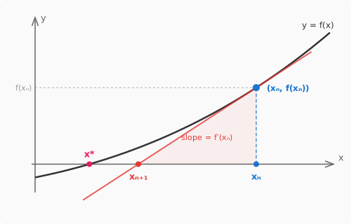
The equation of the tangent line at the point $(x_n,\, f(x_n))$ is
$$y = f(x_n) + f'(x_n)(x - x_n)$$and the point where this tangent line intersects the $x$-axis ($y=0$) is $x_{n+1}$.

Animation: Convergence in Action
The animation below shows how Newton's method converges from the initial value $x_0 = 3.5$ to the root $x^* \approx 2.095$.
Derivation of the Formula
The equation of the tangent line at $(x_n, f(x_n))$ can be written as:
$$y - f(x_n) = f'(x_n)(x - x_n)$$Setting $y = 0$ to find where this tangent line intersects the $x$-axis:
$$0 - f(x_n) = f'(x_n)(x - x_n)$$ $$x = x_n - \dfrac{f(x_n)}{f'(x_n)}$$This is the next approximation $x_{n+1}$. That is, the iteration formula of Newton's method arises naturally as the $x$-intercept of the tangent line.
4. Quadratic Convergence
Theorem (Quadratic Convergence)
If $f$ is twice continuously differentiable and $x_0$ is taken sufficiently close to a simple root $x^*$ ($f(x^*)=0$, $f'(x^*)\neq 0$), then Newton's method converges quadratically. That is, for the constant $C = \dfrac{|f''(x^*)|}{2|f'(x^*)|}$,
holds asymptotically (for large $n$).
This means that the next error is proportional to the square of the current error, multiplied by the constant $C$. For example, if the current error is $10^{-3}$, the next error is approximately $C \times (10^{-3})^2 = C \times 10^{-6}$. The number of correct digits roughly doubles with each iteration, which is why this is called "quadratic" convergence.
Proof
Step 1 (Taylor expansion): Expand $f(x^*)$ in a Taylor series about $x = x_n$ up to first order. Since $f$ is twice continuously differentiable, with the Lagrange form of the remainder as the last term,
$$f(x^*) = f(x_n) + f'(x_n)(x^* - x_n) + \dfrac{f''(\xi_n)}{2}(x^* - x_n)^2$$where $\xi_n$ is some point between $x_n$ and $x^*$. Since $x^*$ is a root ($f(x^*) = 0$),
$$f(x_n) + f'(x_n)(x^* - x_n) + \dfrac{f''(\xi_n)}{2}(x^* - x_n)^2 = 0 \tag{*}$$Step 2 (eliminate $f(x_n)$): Rearranging Newton's iteration formula $x_{n+1} = x_n - \dfrac{f(x_n)}{f'(x_n)}$ gives
$$f(x_n) = f'(x_n)(x_n - x_{n+1})$$Substituting into $(*)$:
$$f'(x_n)(x_n - x_{n+1}) + f'(x_n)(x^* - x_n) + \dfrac{f''(\xi_n)}{2}(x^* - x_n)^2 = 0$$Step 3 (simplify): Factoring $f'(x_n)$ from the first two terms,
$$f'(x_n)\bigl[(x_n - x_{n+1}) + (x^* - x_n)\bigr] + \dfrac{f''(\xi_n)}{2}(x^* - x_n)^2 = 0$$The bracketed expression simplifies to $(x_n - x_{n+1}) + (x^* - x_n) = x^* - x_{n+1}$, so
$$f'(x_n)(x^* - x_{n+1}) + \dfrac{f''(\xi_n)}{2}(x^* - x_n)^2 = 0$$Step 4 (error recurrence): Since $f'(x_n) \neq 0$ (guaranteed when $x^*$ is a simple root and $x_n$ is sufficiently close), dividing both sides by $f'(x_n)$ gives
$$x^* - x_{n+1} = -\dfrac{f''(\xi_n)}{2f'(x_n)}(x^* - x_n)^2$$Reversing signs,
$$x_{n+1} - x^* = \dfrac{f''(\xi_n)}{2f'(x_n)}(x_n - x^*)^2$$Now let $\left|\dfrac{f''(\xi)}{2f'(x)}\right| \le K$ for $\xi, x$ in a neighborhood $I$ of $x^*$, and take $x_0 \in I$ with $K|x_0 - x^*| < 1$. Then $|x_{n+1} - x^*| \le K|x_n - x^*|^2 \le (K|x_0 - x^*|)\,|x_n - x^*|$, so the error decreases monotonically, $x_n$ stays in $I$, and $x_n \to x^*$. Hence $\xi_n \to x^*$ as well, so with $C = \dfrac{|f''(x^*)|}{2|f'(x^*)|}$,
$$|x_{n+1} - x^*| \approx C \cdot |x_n - x^*|^2 \quad \blacksquare$$Meaning of Quadratic Convergence
Since the error decreases quadratically, the number of correct digits approximately doubles with each iteration.
Example: $10^{-2} \to 10^{-4} \to 10^{-8} \to 10^{-16}$

5. Example: Computing $\sqrt{2}$
Applying Newton's Method to $f(x) = x^2 - 2$
Since $f'(x) = 2x$, the iteration formula becomes:
$$x_{n+1} = x_n - \dfrac{x_n^2 - 2}{2x_n} = \dfrac{1}{2}\!\left(x_n + \dfrac{2}{x_n}\right)$$Starting from the initial value $x_0 = 1$:
| $n$ | $x_n$ | Error $|x_n - \sqrt{2}|$ | Correct digits |
|---|---|---|---|
| 0 | 1.000000000 | 4.14 × 10⁻¹ | 0 |
| 1 | 1.500000000 | 8.58 × 10⁻² | 1 |
| 2 | 1.416666667 | 2.45 × 10⁻³ | 2 |
| 3 | 1.414215686 | 2.12 × 10⁻⁶ | 5 |
| 4 | 1.414213562 | 1.59 × 10⁻¹² | 11 |
In just 4 iterations, 11 digits of accuracy are obtained. The progression of correct digits 0 → 1 → 2 → 5 → 11, approximately doubling each time, demonstrates the power of quadratic convergence.
Python implementation
def newton(f, fp, x0, tol=1e-10, max_iter=100):
    """Solve f(x) = 0 by Newton's method.

    Args:
        f, fp: function and its derivative
        x0:    initial guess
        tol:   tolerance applied to both |f(x)| and |Δx|
        max_iter: maximum number of iterations
    Returns:
        (root, iters)
    Raises:
        ValueError: derivative is too close to zero
        RuntimeError: no convergence within max_iter
    """
    x = x0
    for i in range(max_iter):
        fx = f(x)
        fpx = fp(x)
        if abs(fpx) < 1e-14:
            raise ValueError(f"derivative too small at x={x}")
        x_next = x - fx / fpx
        if abs(x_next - x) < tol and abs(f(x_next)) < tol:
            return x_next, i + 1
        x = x_next
    raise RuntimeError(f"did not converge in {max_iter} iterations")

# Example: compute sqrt(2)
root, iters = newton(lambda x: x*x - 2, lambda x: 2*x, x0=1.0)
print(root, iters)  # 1.4142135623730951 5
Implementation notes
- When the derivative is unavailable in closed form: substitute a finite-difference approximation $f'(x) \approx (f(x+h) - f(x))/h$. With $h$ fixed at about $\sqrt{\varepsilon_{\text{mach}}} \cdot \max(1, |x|)$, the iteration converges practically as fast as Newton's method (strictly it is linear, but with a rate proportional to $h$ and therefore tiny). Taking $h$ as the difference $x_{n-1} - x_n$ from the previous iterate gives the secant method, with convergence order $\varphi \approx 1.618$.
- Combine stopping criteria: $|f(x_n)| < \delta$ alone underestimates the error on flat functions; $|x_{n+1}-x_n| < \varepsilon$ alone never triggers on divergence. The robust choice is both criteria plus a hard iteration cap (the implementation above does this).
- Use relative tolerances: when $|x^*|$ is large, switch to $|x_{n+1}-x_n| < \varepsilon (|x_n| + 1)$ so the test is scale-invariant.
6. Multivariable Newton's Method
For a system of nonlinear equations $\mathbf{f}(\mathbf{x}) = \mathbf{0}$ ($\mathbf{x} \in \mathbb{R}^n$), the iteration formula becomes
(provided $J(\mathbf{x}_n)$ is nonsingular), where $J(\mathbf{x})$ is the Jacobian matrix
$$J(\mathbf{x}) = \begin{pmatrix} \dfrac{\partial f_1}{\partial x_1} & \cdots & \dfrac{\partial f_1}{\partial x_n} \\ \vdots & \ddots & \vdots \\ \dfrac{\partial f_n}{\partial x_1} & \cdots & \dfrac{\partial f_n}{\partial x_n} \end{pmatrix}$$Although the iteration formula involves $J^{-1}$, in practice one does not compute the inverse matrix explicitly. Instead, one solves the linear system
$$J(\mathbf{x}_n)\,\Delta\mathbf{x} = -\mathbf{f}(\mathbf{x}_n)$$via LU decomposition or similar methods, and updates $\mathbf{x}_{n+1} = \mathbf{x}_n + \Delta\mathbf{x}$. There are two main reasons for avoiding the explicit inverse:
- Numerical stability: Computing the inverse is susceptible to catastrophic cancellation, whereas solving the linear system directly via LU decomposition yields higher accuracy.
- Memory efficiency: The inverse is a full $n \times n$ dense matrix that must be stored, whereas LU decomposition works in-place and produces $\Delta\mathbf{x}$ directly.
Since $J(\mathbf{x}_n)$ changes at every iteration, the LU factorization must be recomputed each time.
7. Convergence Conditions and Failure Cases
Sufficient Conditions for Convergence
- $f(x^*) = 0$ and $f'(x^*) \neq 0$ (simple root).
- $f$ is twice continuously differentiable in a neighborhood of the root.
- The initial value $x_0$ is sufficiently close to the root.
Failure Cases
- Multiple roots: When $f'(x^*)=0$, convergence degrades to linear. If the multiplicity $m$ is known, the modified Newton's method $x_{n+1} = x_n - m\,f(x_n)/f'(x_n)$ restores quadratic convergence. When $m$ is unknown, one can apply Newton's method to $u(x) = f(x)/f'(x)$ instead, whose roots are all simple.
- Zero (or very small) derivative: If $f'(x_n) = 0$ the iteration is undefined, and if $f'(x_n) \approx 0$ then $x_{n+1}$ is thrown far away. For functions whose $|f'|$ is large far away, such as polynomials, the iterates often come back and converge, but for functions whose tangent flattens far away, such as $\arctan x$, the method diverges (Figure 4 (b)).
- Periodic oscillation: For example, with $f(x) = x^3 - 2x + 2$ and $x_0 = 0$, the iterates oscillate as $x_0 \to 1 \to 0 \to 1 \to \cdots$.
Numerical example of periodic oscillation
With $f(x) = x^3 - 2x + 2$, $f'(x) = 3x^2 - 2$, and $x_0 = 0$:
$$x_1 = 0 - \dfrac{f(0)}{f'(0)} = 0 - \dfrac{2}{-2} = 1$$ $$x_2 = 1 - \dfrac{f(1)}{f'(1)} = 1 - \dfrac{1}{1} = 0$$so $x_3 = 1, x_4 = 0, \ldots$ and the iterates are trapped in a period-2 limit cycle, never reaching the root $x^* \approx -1.7693$. Practical remedies: (i) change the initial value substantially (e.g., $x_0 = -1$ or $x_0 = 0.5$; this cycle is superattracting for the Newton map $N(x) = x - f(x)/f'(x)$, with $N'(0)N'(1) = 0$, so a small perturbation such as $x_0 = 0.1$ falls back into the same oscillation), (ii) detect a repeated visit and switch algorithms, (iii) apply damped Newton ($\alpha < 1$) to break the cycle.
Improved Methods and Practical Remedies
Damped Newton's method ($x_{n+1} = x_n - \alpha_n\, f(x_n)/f'(x_n)$, where $\alpha_n$ is determined by line search) guarantees a monotone decrease of $|f|$ and suppresses divergence and oscillation, but this alone does not guarantee convergence to a root (for example, $f(x) = x e^{-x^2}$ started at $x_0 = 2$ escapes to $x \to \infty$ while decreasing $|f|$). If $f$ is continuous and a sign-changing interval $[a, b]$ is known, combining with the bisection method, falling back to bisection while keeping that interval, guarantees convergence.
Kantorovich's convergence theorem (reference)
Kantorovich's theorem (1948) for the multivariable Newton's method gives a powerful sufficient condition: whenever the product of $\|J(x_0)^{-1} f(x_0)\|$, $\|J(x_0)^{-1}\|$, and the Lipschitz constant of the Jacobian at $x_0$ is small enough, it guarantees existence, uniqueness, and convergence simultaneously. The univariate specialization quantifies how "close" $x_0$ must be to the root. See Ortega-Rheinboldt (1970) for details.
Practical Remedies
- Use the bisection method to narrow down an approximate range, then apply Newton's method.
- Limit the step size when $|f'(x_n)|$ is too small.
- Set an upper bound on the number of iterations.
8. Comparison with the Bisection Method
| Bisection Method | Newton's Method | |
|---|---|---|
| Convergence rate | First-order (linear) | Second-order (quadratic) |
| Required information | $f(x)$ only | $f(x)$ and $f'(x)$ |
| Convergence guarantee | Always converges (if $f$ is continuous and the initial interval has a sign change) | Depends on initial value |
| Typical iterations | 20–50 | 5–10 |
9. Advanced Topics and Related Methods
Below are advanced topics related to Newton's method.
Classical square-root algorithms (the Babylonian and Heron's methods)
The recurrence $x_{n+1} = \dfrac{1}{2}\!\left(x_n + \dfrac{2}{x_n}\right)$ for $\sqrt{2}$ seen in §5 is a special case of the general form $x_{n+1} = \dfrac{1}{2}\!\left(x_n + \dfrac{a}{x_n}\right)$ obtained by applying Newton's method to $f(x) = x^2 - a$. This coincides exactly with the classical Babylonian method (ancient Mesopotamia) and Heron's method (described by Heron of Alexandria in the 1st century) for computing square roots. Newton's method can be regarded as a generalization of such individual root-extraction algorithms to a local iterative method for differentiable equations $f(x) = 0$.
The Newton fractal (basins of attraction)
Applying Newton's method to a function on the complex plane (the classic example being $z^3 - 1 = 0$) and coloring each initial value $z_0$ according to which root it converges to produces a self-similar figure called the Newton fractal. The set of initial values converging to a given root is called that root's basin of attraction, and when there are three or more roots (e.g. $z^3 - 1$) the boundaries between basins have a fractal structure (for $z^2 - 1$ the boundary is a straight line, the imaginary axis). This visually demonstrates sensitivity to the initial value—a tiny change can lead to convergence to a completely different root—and is a striking example of how the global behavior of Newton's method is generally hard to predict.

Higher-order methods (Halley's method)
Using the second derivative $f''$ as well, one can construct iterations with a higher order of convergence than Newton's method. A representative example is Halley's method, which converges cubically:
$$x_{n+1} = x_n - \dfrac{2\, f(x_n)\, f'(x_n)}{2\, f'(x_n)^2 - f(x_n)\, f''(x_n)}$$The cost per step increases, but it is advantageous when very high accuracy is required or when $f''$ is cheap to evaluate. Newton's method (quadratic convergence) is the most basic case of such higher-order iterations.
Quasi-Newton methods (derivative-approximating variants)
When the derivative or Jacobian is difficult or expensive to compute, variants that approximate them are used. In one dimension, the secant method approximates $f'$ by a finite difference (order of convergence $\varphi \approx 1.618$); in several dimensions, quasi-Newton methods approximate and update the Jacobian at each iteration. The classic instance is Broyden's method (1965), which performs a low-rank update of the Jacobian approximation from the change in function values at each step. The BFGS method, widely used in optimization, is also a quasi-Newton method.
10. Summary
- Newton's method iteration formula: $x_{n+1} = x_n - \dfrac{f(x_n)}{f'(x_n)}$
- It is a graphical method that uses the intersection of the tangent line with the $x$-axis as the next approximation.
- Quadratic convergence: the number of correct digits approximately doubles with each iteration.
- Computation of the derivative $f'(x)$ is required.
- The choice of initial value is critical, and convergence is not guaranteed in all cases.
- Extension to multiple variables requires the Jacobian matrix and solving a linear system.
11. Frequently Asked Questions
Q1. What is Newton's method?
It is a technique for iteratively finding roots of a nonlinear equation $f(x)=0$ using tangent-line approximation. The iteration formula is $x_{n+1} = x_n - f(x_n)/f'(x_n)$.
Q2. How fast does Newton's method converge?
Near a simple root, it converges quadratically. That is, the number of correct digits approximately doubles with each iteration. For multiple roots, convergence degrades to linear.
Q3. Can Newton's method fail?
It can fail when the derivative is close to zero, when the initial value is too far from the root, or when periodic oscillation occurs. Damped Newton's method or combining with the bisection method can address these issues.
Q4. Can I see Newton's method convergence as an animation?
This page includes an interactive animation that visualizes the iteration: starting from an initial value, drawing the tangent line, and taking its intersection with the $x$-axis as the next approximation. You can observe how quadratic convergence rapidly increases the number of correct digits.
Q5. What is the Newton fractal?
It is an image obtained by applying Newton's method to a function on the complex plane (e.g. $z^3-1$) and coloring each initial value according to which root it converges to. When there are three or more roots, the boundaries between the roots' basins of attraction have a fractal structure, demonstrating sensitivity to the initial value: a tiny change can lead to a different root.
Q6. Are there iterative methods faster than Newton's method?
Halley's method, which uses the second derivative $f''$, converges cubically and is faster than Newton's method (quadratic). When the derivative is hard to compute, the secant method or quasi-Newton methods (Broyden's method) approximate $f'$ or the Jacobian (BFGS, used in optimization, is a quasi-Newton method that approximates the Hessian).
12. References
- Wikipedia, "Newton's method"
- Wikipedia, "Kantorovich theorem"
- R. L. Burden & J. D. Faires, Numerical Analysis, 10th ed., Cengage, 2016.
- J. Nocedal & S. J. Wright, Numerical Optimization, 2nd ed., Springer, 2006.
- J. M. Ortega & W. C. Rheinboldt, Iterative Solution of Nonlinear Equations in Several Variables, Academic Press, 1970 (the standard reference for multivariate Newton and the Kantorovich theorem).
- L. V. Kantorovich, "Functional analysis and applied mathematics," Uspekhi Mat. Nauk, vol. 3, no. 6, pp. 89--185, 1948 (original Kantorovich convergence theorem).
- N. J. Higham, Accuracy and Stability of Numerical Algorithms, 2nd ed., SIAM, 2002 (Chapter 3 on numerical stability of iterations and stopping-criterion pitfalls).
- Wikipedia, "Newton fractal" (basins of attraction on the complex plane).
- Wikipedia, "Quasi-Newton method" (Broyden, BFGS).
Implementation in sangi
The algorithm in this article is available in sangi's newton_raphson / newton_raphson_nd.