What is a parametric curve?

A parametric curve is a smooth map γ: I → R^n (n ≥ 2) from an open interval I ⊂ R. As the parameter t varies, γ(t) traces out a curve in space. In differential geometry, plane curves (n = 2) and space curves (n = 3) are the most commonly studied.

What is a regular curve?

A regular curve is a parametric curve that is C^1 (at least once continuously differentiable) and whose velocity vector γ'(t) is nonzero for every parameter value t. Regularity ensures that the tangent direction is uniquely determined at each point, ruling out cusps and stationary points.

What is reparametrization?

Reparametrization is the process of replacing the parameter of a curve using a smooth function φ: J → I with φ'(s) ≠ 0, giving a new parametric curve γ̃(s) = γ(φ(s)). Geometrically, the same curve is traversed, but at a different speed. If φ' > 0 the orientation is preserved; if φ' < 0 the orientation is reversed.

Chapter 1: Parametric Curves

Curve Definitions, Regular Curves, and Reparametrization

Introduction

In differential geometry, curves are expressed using a "parameter." This allows each point on a curve to be specified by a single variable, and the properties of the curve can then be studied using the tools of calculus.

Definition of a Curve

Definition: Parametric Curve

A smooth map from an open interval $I \subset \mathbb{R}$ to $\mathbb{R}^n$ ($n \geq 2$),

$$\gamma: I \to \mathbb{R}^n, \quad t \mapsto \gamma(t) = (\gamma_1(t), \gamma_2(t), \ldots, \gamma_n(t))$$

is called a parametric curve. In differential geometry, the cases $n = 2$ (plane curves) and $n = 3$ (space curves) are most commonly studied.

A parametric curve: a point t in the interval [a, b] corresponds to a point γ(t) on the curve, with the tangent vector γ'(t) drawn

Figure 1: A parametric curve — each point $t$ in the interval $[a, b]$ corresponds to a point $\gamma(t)$ on the curve. The red arrow represents the tangent vector $\gamma'(t)$.

Examples: Circle and Parabola

Example 1: Unit Circle

$$\gamma(t) = (\cos t, \sin t), \quad t \in [0, 2\pi]$$

The parameter $t$ corresponds to the angle (in radians).

Parametric representation of the unit circle γ(t) = (cos t, sin t), where the parameter t corresponds to the angle

Figure 2: Parametric representation of the unit circle — the parameter $t$ corresponds to the angle, and the point $\gamma(t)$ moves counterclockwise around the circle.

Example 2: Parabola

$$\gamma(t) = (t, t^2), \quad t \in \mathbb{R}$$

This is a parametric representation of the graph $y = x^2$.

Parametric representation of the parabola γ(t) = (t, t²), with the vertex at t=0 and the tangent vector drawn at t=1

Figure 3: Parametric representation of the parabola — the graph $y = x^2$ is expressed as $\gamma(t) = (t, t^2)$. The red arrow shows the tangent vector $\gamma'(1) = (1, 2)$ at $t = 1$.

Example 3: Helix

$$\gamma(t) = (a\cos t, a\sin t, bt), \quad t \in \mathbb{R}$$

For $a > 0$ and $b \neq 0$, this represents a helix winding around a cylinder.

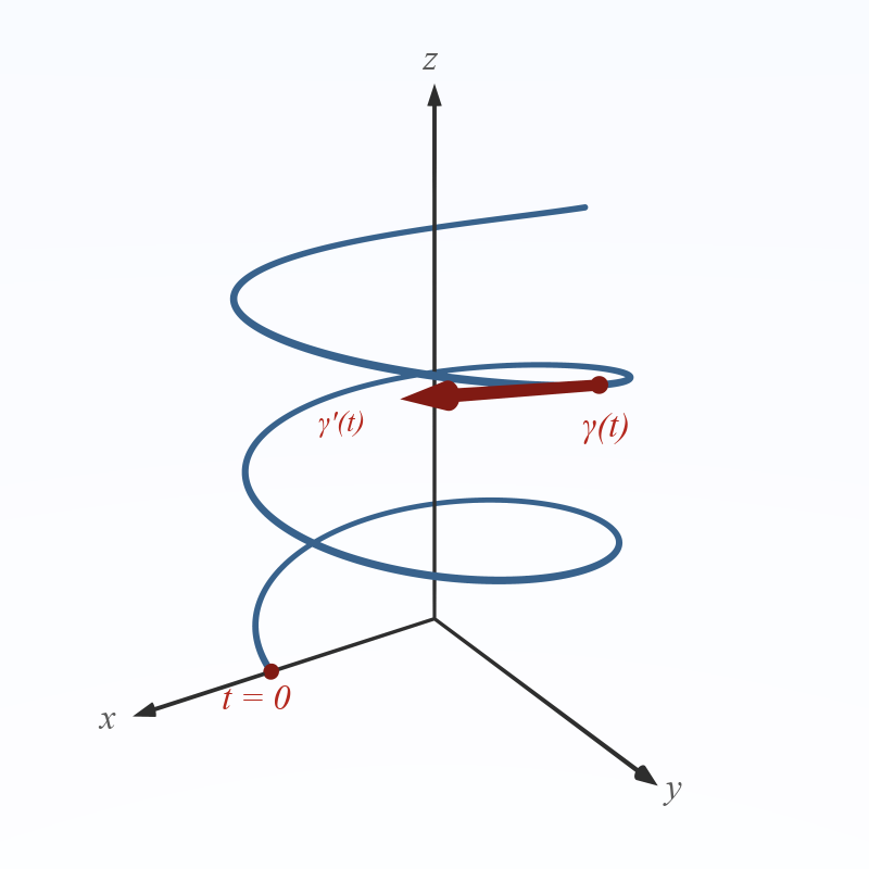
3D ray-traced rendering of the helix γ(t) = (a cos t, a sin t, bt), showing the spiral curve and the tangent vector γ'(t)

Figure 4: Helix — a spiral curve $\gamma(t) = (a\cos t, a\sin t, bt)$ ascending along the $z$-axis. The red arrow represents the tangent vector $\gamma'(t)$.

Regular Curves

Definition: Regular Curve

A parametric curve $\gamma: I \to \mathbb{R}^n$ is said to be regular if $\gamma$ is of class $C^1$ (at least once continuously differentiable) and for all $t \in I$,

$$\gamma'(t) \neq \mathbf{0}$$

The vector $\gamma'(t)$ is called the velocity vector.

Regularity imposes two conditions: (1) differentiability (no cusps), and (2) the derivative never vanishes (no stationary points). This ensures that the tangent direction is uniquely determined at every point of the curve.

Meaning of the Velocity Vector

$\gamma'(t) = \left(\frac{d\gamma_1}{dt}, \frac{d\gamma_2}{dt}, \ldots, \frac{d\gamma_n}{dt}\right)$ represents the tangent direction of the curve at parameter $t$. If the parameter $t$ is interpreted as time, then $\gamma'(t)$ corresponds to the velocity of a particle, and regularity means "the particle is always in motion."

Example: A Non-Regular Curve

$$\gamma(t) = (t^3, t^2), \quad t \in \mathbb{R}$$

Since $\gamma'(t) = (3t^2, 2t)$, we have $\gamma'(0) = (0, 0)$ at $t = 0$. Therefore the curve is not regular at $t = 0$.

This curve has a cusp at the origin.

The non-regular curve γ(t) = (t³, t²) with a cusp at the origin where γ'(0) = (0, 0)

Figure 5: A non-regular curve $\gamma(t) = (t^3, t^2)$ — the curve has a cusp at the origin. At $t = 0$, $\gamma'(0) = \mathbf{0}$, and the tangent direction is undefined.

Reparametrization

The same curve can be expressed using different parameters. For example, given the unit circle $\gamma(t) = (\cos t, \sin t)$, setting $\phi(s) = s^2$ yields

$$\tilde{\gamma}(s) = \gamma(s^2) = (\cos s^2, \sin s^2)$$

which traces the same circle but at a different speed. While $\gamma$ traverses the circle at constant speed, $\tilde{\gamma}$ moves slowly when $s$ is small and accelerates as $s$ increases. Geometrically it is the same curve, but the "rate of traversal" differs. (Note: since $\phi'(s) = 2s$ vanishes at $s = 0$, this is strictly a valid reparametrization only for $s > 0$.)

Comparison of reparametrizations: left shows evenly spaced nodes with the original parameter; right shows nodes clustered near the start with the s² parameter

Figure 6: Comparison of reparametrizations — the same unit circle traversed with parameter $t$ (left) and $s^2$ (right). Evenly spaced values of $t$ produce evenly spaced nodes on the circle, whereas evenly spaced values of $s$ cluster nodes near the starting point, with spacing increasing along the way.

Definition: Reparametrization

If $\phi: J \to I$ is smooth with $\phi'(s) \neq 0$, then $\tilde{\gamma} = \gamma \circ \phi$ is called a reparametrization of $\gamma$.

$$\tilde{\gamma}(s) = \gamma(\phi(s))$$

Proposition: Velocity under Reparametrization

If $\tilde{\gamma} = \gamma \circ \phi$, then by the chain rule,

$$\tilde{\gamma}'(s) = \gamma'(\phi(s)) \cdot \phi'(s)$$

Therefore, if $\gamma$ is regular and $\phi' \neq 0$, then $\tilde{\gamma}$ is also regular.

When $\phi' > 0$, the reparametrization is said to be "orientation-preserving"; when $\phi' < 0$, it is "orientation-reversing."

Summary

A curve is defined as a smooth map from an interval into a space.
A regular curve is one whose velocity vector is nonzero at every point.
The same curve can be expressed with different parameters (reparametrization).
In differential geometry, regular curves are the fundamental objects of study.