Chapter 1: Riemannian Geometry
Differential geometry of curved spaces
Goal of this page
Study the Levi-Civita connection and the curvature tensor in detail, and understand the central concepts of Riemannian geometry such as Jacobi fields and comparison theorems.
Riemannian geometry is the branch of differential geometry that equips each point of a curved space with an inner product (a Riemannian metric) and, on that basis, defines distance, angle, curvature, and geodesics (shortest paths) intrinsically within differential geometry. It generalizes Euclidean geometry to surfaces and manifolds, and forms the mathematical foundation of general relativity. Below we look in turn at its core ingredients: the connection, curvature, Jacobi fields, and comparison theorems.
1. The Levi-Civita Connection
For a Riemannian manifold $(M, g)$ there exists a unique connection $\nabla$ satisfying:
- Torsion-free: $\nabla_X Y - \nabla_Y X = [X, Y]$
- Metric-compatible: $X g(Y, Z) = g(\nabla_X Y, Z) + g(Y, \nabla_X Z)$
The covariant derivative of a vector field $Y$ in the direction $X$:
$$\nabla_X Y = \displaystyle\sum_k \left( X(Y^k) + \displaystyle\sum_{i,j} \Gamma^k_{ij} X^i Y^j \right) \dfrac{\partial}{\partial x^k}$$On flat space, vectors at two separated points can be compared by subtracting their components directly. But on a curved space the coordinate basis vectors $\partial/\partial x^k$ themselves change direction from point to point. The covariant derivative corrects for this change of basis using the Christoffel symbols $\Gamma^k_{ij}$, extracting only “how much the vector field itself changed.” The condition $\nabla_X Y = 0$ means that “$Y$ is kept parallel in the direction $X$,” which is the definition of parallel transport.
The Levi-Civita connection is uniquely determined by the metric $g_{ij}$:
$$\Gamma^k_{ij} = \frac{1}{2} \sum_l g^{kl}\left( \frac{\partial g_{jl}}{\partial x^i} + \frac{\partial g_{il}}{\partial x^j} - \frac{\partial g_{ij}}{\partial x^l} \right)$$Here $g^{kl}$ is the inverse of the metric tensor $g_{ij}$. This expression follows uniquely from the two conditions of being torsion-free and metric-compatible.
Writing the plane in polar coordinates $(r, \theta)$, the metric is $ds^2 = dr^2 + r^2\, d\theta^2$, i.e. $g_{rr}=1,\ g_{\theta\theta}=r^2,\ g_{r\theta}=0$, with inverse metric $g^{rr}=1,\ g^{\theta\theta}=1/r^2$. Only $\partial_r g_{\theta\theta} = 2r$ is nonzero, so
$$\Gamma^r_{\theta\theta} = -\tfrac{1}{2} g^{rr}\,\partial_r g_{\theta\theta} = -r,\qquad \Gamma^\theta_{r\theta} = \Gamma^\theta_{\theta r} = \tfrac{1}{2} g^{\theta\theta}\,\partial_r g_{\theta\theta} = \frac{1}{r}$$All other components are $0$. Even though the plane is flat, the Christoffel symbols do not vanish — this reflects not curvature of the space but “distortion of the curvilinear coordinates.” Indeed, computing the curvature tensor of the next section gives all zeros, confirming that the plane is flat.
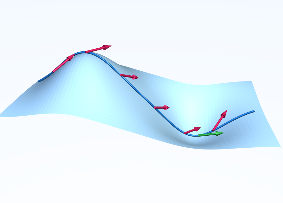
Once a connection is fixed, we can define parallel transport of a vector along a curve. Writing the transported tangent vector as $V$, the curve as $\gamma$, and its tangent (velocity vector) as $\gamma'$, the vector $V$ is carried while satisfying $\nabla_{\gamma'} V = 0$. Here “parallel” means that it does not rotate relative to the surface (an inhabitant of the surface always sees it pointing the same way); on a plane this coincides with ordinary parallel translation that carries the vector without changing its direction. When the surface is curved, however, the tangent plane itself tilts, so viewed from the surrounding 3-dimensional space $V$ appears to change direction little by little. This “apparent rotation” is precisely the manifestation of curvature (see the figure below).
 $V$
$\gamma'$
$\gamma$
$V$
$\gamma'$
$\gamma$
2. Properties of the Curvature Tensor
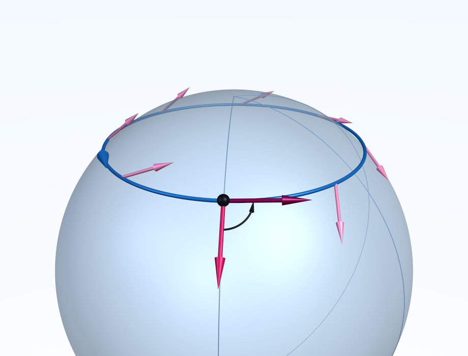
Second covariant derivatives do not commute in general. That discrepancy $\nabla_X\nabla_Y - \nabla_Y\nabla_X - \nabla_{[X,Y]}$ is the curvature $R(X,Y)$. Geometrically it works as follows. In Figure 1 we carried $V$ along an open curve; here we parallel transport the same tangent vector $V$ once around a closed curve through a point $P$ and back to $P$. Calling the returned vector $V'$, on a curved space $V'$ is rotated from the original $V$ by an angle $\Delta\theta$ (holonomy), and that rotation angle $\Delta\theta$ equals the total curvature enclosed by the loop. If the curvature is zero the rotation is zero too — on flat space parallel transport is path-independent (see the figure below).
 $V$
$V'$
$P$
$\Delta\theta$
$V$
$V'$
$P$
$\Delta\theta$
Parallel transport around a closed curve is a rotation of the tangent plane, so the returned vector is $V' = R_{\Delta\theta}\,V$ with unchanged length ($|V'|=|V|$). Hence the angle formed by $V$ (start) and $V'$ (after one loop) is exactly the rotation angle:
$$\Delta\theta = \cos^{-1}\!\frac{\langle V',\,V\rangle}{|V'|\,|V|} = \iint_\Sigma K\, dA$$The left equality is the geometric fact that “$V'$ is $V$ rotated by $\Delta\theta$”; the right equality is the local Gauss-Bonnet theorem (rotation angle = total curvature enclosed). However, $\cos^{-1}$ returns a value in $[0,\pi]$, so this identity holds directly only when $0 \le \Delta\theta \le \pi$. When the total curvature is large and $\Delta\theta$ exceeds $\pi$, or when the orientation (sign) of the rotation is also taken into account, $\iint_\Sigma K\,dA$ carries the complete information ($\cos^{-1}$ folds back to the principal value).
- $R(X, Y) = -R(Y, X)$
- $g(R(X, Y)Z, W) = -g(R(X, Y)W, Z)$
- $g(R(X, Y)Z, W) = g(R(Z, W)X, Y)$
- Bianchi identity: $R(X, Y)Z + R(Y, Z)X + R(Z, X)Y = 0$
The sectional curvature of a 2-dimensional subspace $\sigma = \text{span}\{X, Y\}$:
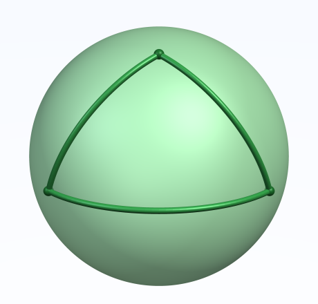
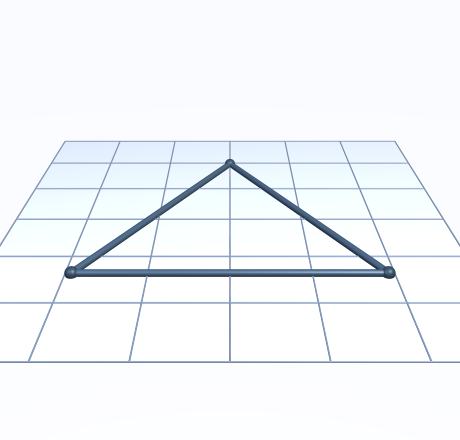
$$K(\sigma) = \dfrac{g(R(X, Y)Y, X)}{g(X, X)g(Y, Y) - g(X, Y)^2}$$Choosing a 2-dimensional plane $\sigma$ inside the tangent space, $K(\sigma)$ is the (Gaussian) curvature of the surface swept out by the geodesics in those directions. The sign determines the geometry: $K>0$ is spherical (geodesics converge; the angle sum of a geodesic triangle exceeds $\pi$), $K=0$ is flat, and $K<0$ is hyperbolic (geodesics diverge; the angle sum is less than $\pi$).
Angle sum $ > \pi$ (sphere)
Angle sum $ = \pi$ (plane)
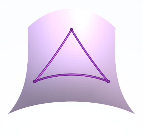
Angle sum $ < \pi$ (hyperbolic)
The sphere $S^2_r$ of radius $r$ has constant sectional curvature $K = 1/r^2$ in every 2-dimensional direction. The larger the radius, the smaller the curvature, approaching the plane ($K\to 0$) as $r\to\infty$. On the other hand, the hyperbolic plane $\mathbb{H}^2$ is a constant-curvature space with $K=-1$. These three — the sphere ($K>0$), the Euclidean plane ($K=0$), and the hyperbolic plane ($K<0$) — are the representatives of constant-curvature spaces, corresponding to the three triangles in Figure 3.
3. Jacobi Fields
A vector field $J$ arising from a variation of geodesics that satisfies the Jacobi equation:
$$\nabla_{\gamma'}^2 J + R(J, \gamma')\gamma' = 0$$is called a Jacobi field.
Launching geodesics from a single point with slightly varying directions, they separate and then re-gather. The Jacobi field $J$ measures the gap between neighboring geodesics, and its growth is governed by the Jacobi equation. In two dimensions the equation takes the form $J'' + K J = 0$, where the sectional curvature $K$ plays the role of a spring constant. If $K>0$, $J$ oscillates and returns to $0$ (a conjugate point — the re-focusing of geodesics); if $K<0$, it diverges exponentially.
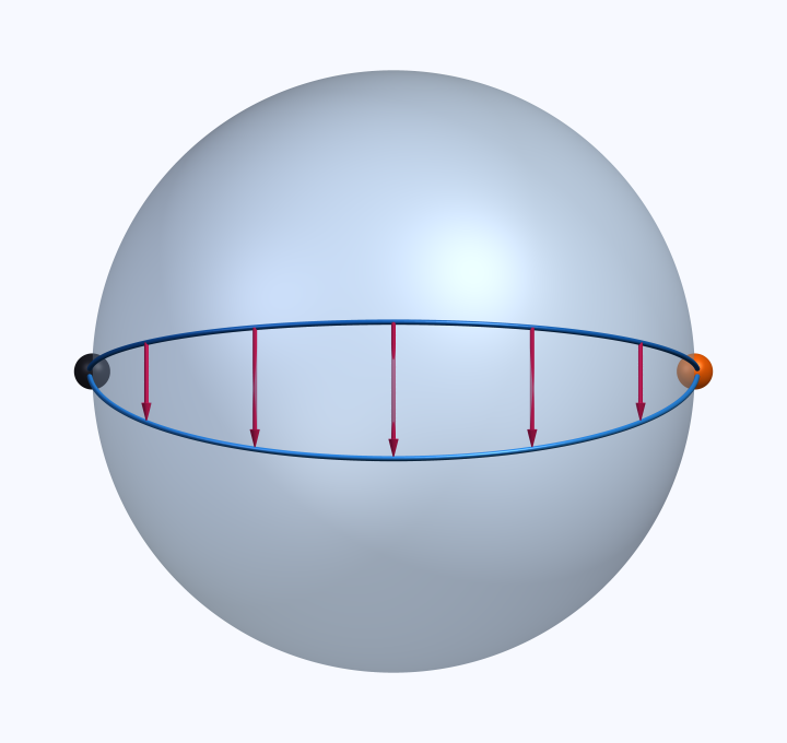 $p$
$q$
Reference geodesic $\gamma$
Neighbor geodesic
$J(t)$
$p$
$q$
Reference geodesic $\gamma$
Neighbor geodesic
$J(t)$
A value $t_0 > 0$ for which a nonzero Jacobi field $J \neq 0$ has $J(0) = 0$ and $J(t_0) = 0$ is called a conjugate point.
Beyond a conjugate point the geodesic is no longer shortest.
On the unit sphere $S^2$ ($K=1$), the Jacobi equation along a great circle is $J'' + J = 0$. The solution with $J(0)=0$ is $J(t) = \sin t$, which returns to $0$ at $t = \pi$. That is, geodesics (meridians) leaving the north pole meet again at the antipodal point (the point diametrically opposite through the center — the south pole for the north pole) at distance $\pi$, and that is the conjugate point. For a sphere of radius $r$ the distance to the conjugate point is $\pi r$ (the antipode). The way geodesics open up and re-gather at the conjugate point is exactly the lens shape of Figure 4 (Figure 4 uses a flattened surface of revolution to make $p, q$ easy to see).
4. Comparison Theorems
If the Ricci curvature satisfies $\text{Ric} \geq (n-1)\kappa > 0$, then $M$ is compact and
$$\text{diam}(M) \leq \dfrac{\pi}{\sqrt{\kappa}}$$If the Ricci curvature has a positive lower bound, then every geodesic, in whatever direction, reaches a conjugate point within a finite distance and is no longer shortest beyond it. Hence the manifold cannot extend infinitely: its diameter is bounded by $\pi/\sqrt{\kappa}$ and it is compact. Picture curvature acting as a “restoring force that pulls geodesics back”; the oscillation (re-focusing) of the Jacobi equation $J''+KJ=0$ from the previous section is its essence.
The sphere $S^2$ of radius $r$ has $\mathrm{Ric} = (n-1)/r^2$ ($n=2$), i.e. $\kappa = 1/r^2$. The Bonnet-Myers bound is $\mathrm{diam} \le \pi/\sqrt{\kappa} = \pi r$. The actual diameter of the sphere (half the length of a great circle) is exactly $\pi r$, so equality holds. The sphere is the typical equality case of the comparison theorem.
For a compact 2-dimensional Riemannian manifold $M$:
$$\displaystyle\int_M K\, dA = 2\pi \chi(M)$$The Gauss-Bonnet theorem asserts that integrating the local bending $K$ over the whole surface gives a total that depends only on the topology of the surface (the Euler characteristic $\chi$). However bumpy the deformation, the total curvature is invariant. The sphere has $\chi=2$ with $\int K\,dA = 4\pi$; the torus (doughnut) has $\chi=0$ with $\int K\,dA = 0$ — the positive curvature on the outside and the negative curvature on the inside (the hole side) cancel exactly.
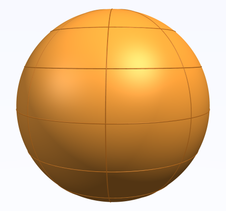 $K>0$
$K>0$
$\int K\,dA = 4\pi$
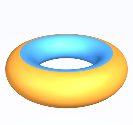 $K>0$
$K \lt 0$
$K>0$
$K \lt 0$
$\int K\,dA = 0$ (positive + negative cancel)
Applying the Gauss-Bonnet theorem to a geodesic triangle, the difference between the angle sum and $\pi$ (the angular excess) equals the total curvature inside:
$$(\alpha+\beta+\gamma) - \pi = \iint_{\triangle} K\, dA$$Consider on the unit sphere a triangle whose three sides all meet at right angles (an octant of the sphere): then $\alpha=\beta=\gamma=\pi/2$, so the angular excess is $3\cdot\tfrac{\pi}{2}-\pi = \tfrac{\pi}{2}$. Its area is $1/8$ of the whole sphere $4\pi$, namely $\tfrac{\pi}{2}$, and since $K=1$ the right-hand side is also $\tfrac{\pi}{2}$, so the two sides agree. This quantifies the $K>0$ triangle of Figure 3 (angle sum $>\pi$).
Summary
Key points of this chapter
- Levi-Civita connection: torsion-free + metric-compatible
- Curvature tensor: path-dependence of parallel transport
- Jacobi field: variation of geodesics, conjugate points
- Comparison theorems: deriving global properties from the sign of curvature
This article is a survey overview of the branches of advanced geometry. To study the connection, curvature, Jacobi fields, and comparison theorems covered here chapter by chapter and in more depth — from the Riemannian metric through geodesics, the exponential map, and the curvature tensor — continue to the differential geometry course.
Frequently asked questions
What is Riemannian geometry?
Riemannian geometry is the branch of differential geometry that studies manifolds (Riemannian manifolds) equipped with an inner product (a Riemannian metric) at each point. It lets one define distance, angle, curvature, and geodesics (shortest paths) intrinsically, and forms the mathematical foundation of general relativity.
What is the Levi-Civita connection?
It is the standard (symmetric and metric-compatible) covariant derivative on a Riemannian manifold. It defines parallel transport and characterizes geodesics as curves of zero acceleration. It is expressed in local coordinates by the Christoffel symbols $\Gamma^k_{ij}$ and is used to compute the Riemann curvature tensor.
What is the relationship between the Riemann curvature tensor and the sectional curvature?
The Riemann curvature tensor $R^l{}_{kij}$ is a $(1,3)$-type tensor describing the bending of a Riemannian manifold. The sectional curvature $K(\sigma)$ is the cross-sectional curvature of a 2-dimensional subspace $\sigma$ of the tangent space, given by a particular contraction of the tensor. Constant-curvature spaces (sphere, hyperbolic space, flat space) are the special case where the sectional curvature is constant.