Color Spaces
What Is a Color Space?
A color space is a coordinate system for representing colors numerically. Different color spaces are chosen depending on the application.
RGB Color Space
The RGB color space represents colors by additive mixing of three primary colors: Red, Green, and Blue.
RGB Cube
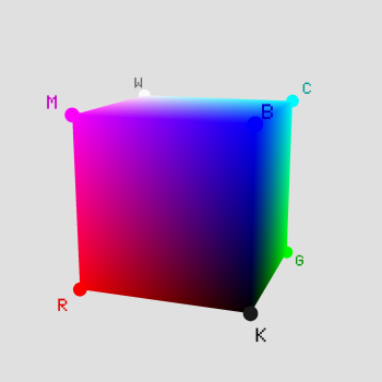
Additive Mixing
R, G, B ∈ [0, 255] (8-bit) Total colors: 256³ ≈ 16.77 million
Light Primaries vs. Pigment Primaries
There are two fundamentally different ways to mix colors.
| Property | Additive (Light Primaries) | Subtractive (Pigment Primaries) |
|---|---|---|
| Primaries | R (Red), G (Green), B (Blue) | C (Cyan), M (Magenta), Y (Yellow) |
| Mixing result | Gets brighter (all mixed → white) | Gets darker (all mixed → theoretically black) |
| Principle | Adding light (emission) | Absorbing light (subtracting from reflected light) |
| Applications | Displays, lighting, cameras | Printing (CMYK), paint |
| Relationship | C = G+B (remove red), M = R+B (remove green), Y = R+G (remove blue) Additive and subtractive primaries are complementary |
|
In printing, CMY alone cannot produce true black, so black ink (K: Key) is added, giving CMYK. Computer vision primarily uses additive RGB.
Note: OpenCV stores images in BGR order. Conversion is needed when working with RGB images.
HSV/HSL Color Space
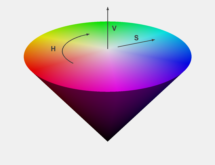
HSV (Hue, Saturation, Value) represents colors in a way that is closer to human perception, making it well-suited for color selection and extraction.
HSV Components
- H (Hue): The type of color. Expressed as 0°–360° (red=0°, green=120°, blue=240°)
- S (Saturation): Color vividness. 0–1 (0=gray, 1=pure color)
- V (Value): Brightness. 0–1 (0=black, 1=maximum brightness)
RGB → HSV Conversion
$$M = \max(R, G, B), \quad m = \min(R, G, B), \quad C = M - m$$ $$V = M, \quad S = \frac{C}{M} \quad (M \neq 0)$$ $$H = 60° \times \begin{cases} (G-B)/C \bmod 6 & \text{if } M=R \\ (B-R)/C + 2 & \text{if } M=G \\ (R-G)/C + 4 & \text{if } M=B \end{cases}$$Applications: Color-based object detection, skin detection, background subtraction, etc. For example, red detection specifies H: 0°–10° or 350°–360°.
OpenCV-specific note: In OpenCV, Hue ranges from 0 to 179 (360° halved to fit in 8 bits), while Saturation and Value range from 0 to 255. When converting from the formulas above, divide H by 2.
YUV / YCbCr Color Space
These color spaces separate luminance (Y) from chrominance. Since human vision is more sensitive to luminance than to color differences, the chrominance channels can be subsampled to reduce data size.
Difference Between YUV and YCbCr
| Property | YUV | YCbCr |
|---|---|---|
| Origin | Analog TV (PAL / NTSC) | Digital video standards |
| Value range | Continuous (analog signal) | Quantized to 0–255 (digital) |
| Applications | Analog broadcast, video signals | JPEG, H.264, MPEG, HDMI |
| Coefficients | Vary by standard (BT.601: SD, BT.709: HD, BT.2020: 4K/8K) | |
YUV and YCbCr are often conflated in literature and libraries, but
OpenCV's COLOR_BGR2YUV and COLOR_BGR2YCrCb perform different conversions.
Modern computer vision primarily uses YCbCr (the digital variant).
RGB → YCbCr Conversion (BT.601)
$$\begin{pmatrix} Y \\ C_b \\ C_r \end{pmatrix} = \begin{pmatrix} 0.299 & 0.587 & 0.114 \\ -0.169 & -0.331 & 0.500 \\ 0.500 & -0.419 & -0.081 \end{pmatrix} \begin{pmatrix} R \\ G \\ B \end{pmatrix} + \begin{pmatrix} 0 \\ 128 \\ 128 \end{pmatrix}$$YCbCr value range: Video standards typically use "studio swing" ranges: Y from 16 to 235, Cb/Cr from 16 to 240.
However, OpenCV's cvtColor uses full range (0–255).
Lab Color Space (CIELAB)
Lab is a perceptually uniform color space designed to match human perception. Euclidean distance in Lab correlates well with perceived color difference, making it widely used for color difference evaluation and color management.
Lab Components
- L: Lightness (0=black, 100=white)
- a: Green (−) to Red (+) axis
- b: Blue (−) to Yellow (+) axis
RGB → Lab Conversion Pipeline
RGB → XYZ (device-independent intermediate) → Lab
The XYZ-to-Lab conversion uses a nonlinear function:
$$L^* = 116\,f\!\left(\frac{Y}{Y_n}\right) - 16, \quad a^* = 500\left[f\!\left(\frac{X}{X_n}\right) - f\!\left(\frac{Y}{Y_n}\right)\right], \quad b^* = 200\left[f\!\left(\frac{Y}{Y_n}\right) - f\!\left(\frac{Z}{Z_n}\right)\right]$$where $f(t) = t^{1/3}$ (when $t > \delta^3$), $\delta = 6/29$. $X_n, Y_n, Z_n$ are the tristimulus values of the white point.
Applications: Color difference calculation ($\Delta E$), color calibration, image segmentation. $\Delta E = \sqrt{(\Delta L^*)^2 + (\Delta a^*)^2 + (\Delta b^*)^2}$ serves as a perceptual color difference metric.
Grayscale Conversion
There are several methods to convert a color image to grayscale:
Luminosity Method — most common
$$Y = 0.299R + 0.587G + 0.114B$$Weights based on human eye sensitivity
Average Method
$$Y = \frac{R + G + B}{3}$$Lightness Method
$$Y = \frac{\max(R,G,B) + \min(R,G,B)}{2}$$Code Example (Python)
import cv2
import numpy as np

# Read image (BGR)
img_bgr = cv2.imread('image.jpg')

# Color space conversions
img_rgb = cv2.cvtColor(img_bgr, cv2.COLOR_BGR2RGB)
img_hsv = cv2.cvtColor(img_bgr, cv2.COLOR_BGR2HSV)
img_ycrcb = cv2.cvtColor(img_bgr, cv2.COLOR_BGR2YCrCb)
img_gray = cv2.cvtColor(img_bgr, cv2.COLOR_BGR2GRAY)
img_lab = cv2.cvtColor(img_bgr, cv2.COLOR_BGR2LAB)

# Extract a specific color using HSV (e.g., red)
lower_red = np.array([0, 100, 100])
upper_red = np.array([10, 255, 255])
mask = cv2.inRange(img_hsv, lower_red, upper_red)
result = cv2.bitwise_and(img_bgr, img_bgr, mask=mask)

# Manual grayscale calculation (luminosity method)
b, g, r = cv2.split(img_bgr)
gray_manual = (0.299 * r + 0.587 * g + 0.114 * b).astype(np.uint8)
Summary
- RGB: The standard for display, based on additive mixing
- HSV/HSL: Closer to human perception, ideal for color extraction
- YUV/YCbCr: Separates luma from chroma, used in video compression
- Lab: Perceptually uniform, optimal for color difference and color management
- Grayscale: Luminance only, widely used as preprocessing for image analysis