MLS stands for Maximum Length Sequence, a class of pseudorandom binary sequences. Its periodic autocorrelation is essentially a unit pulse, which is the property exploited for impulse response measurement.

Impulse Response Measurement Using Time-Reversed MLS

This article is based on a presentation given on 2018-08-25 at the Music Acoustics Committee of the Acoustical Society of Japan, held at NHK Science & Technology Research Laboratories. The DFT appears in the derivation, but no DFT is required at runtime: the impulse response can be measured with ordinary FIR convolution alone.

Introduction

A well-known way to measure the impulse response of a linear time-invariant (LTI) system is to drive it with a $\pm 1$ binary maximum-length sequence (MLS), compute the cross-correlation between input and output efficiently via the Hadamard transform, and apply a scaling correction (Borish & Angell, Kaneda).

Here we take a different route. We first adjust the gain and offset of an MLS so that its DFT magnitude spectrum is unity at every frequency, and then convolve the system's output with one period of the time-reversed signal (which is equivalent to a circular cross-correlation). The impulse response falls out directly as a result.

Definitions

The unit pulse, defined for any integer argument, is given by

$$ \delta(n) = \left\{ \begin{array}{cl} 1, & n=0 \\ 0, & \text{otherwise} \end{array} \right. \tag{1} $$

The same definition applies regardless of the argument symbol ($\delta(n)$, $\delta(k)$, etc.).

The $N$-point DFT and inverse DFT are taken to be

$$ \begin{aligned} \text{DFT} &: X(k) = \sum_{n=0}^{N-1} x(n)\exp\!\left(-2\pi i \frac{nk}{N}\right) \\[6pt] \text{Inverse DFT} &: x(n) = \frac{1}{N}\sum_{k=0}^{N-1} X(k)\exp\!\left(2\pi i \frac{nk}{N}\right) \end{aligned} \tag{2} $$

The autocorrelation of a period-$N$ periodic signal is defined for $0\leq n\lt N$ by

$$ r(n) = \sum_{i=0}^{N-1} x(i)\, x(i+n) \tag{3} $$

Constructing a periodic signal with unit magnitude spectrum at all frequencies

Gain adjustment

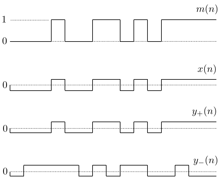
From a binary MLS $m(n)\in\{0,1\}$ of period $N$, build the bipolar periodic waveform

$$ x(n) = \frac{1}{\sqrt{N}}\left\{2\, m(n)-1\right\} \tag{4}\label{xn} $$

which takes the two values $\pm\displaystyle\frac{1}{\sqrt{N}}$. Its periodic autocorrelation is (Kashiwagi)

$$ r(n) = \left\{ \begin{array}{cl} 1, & n=0 \\ -\displaystyle\frac{1}{N}, & \text{otherwise} \end{array} \right. = \left(1+\frac{1}{N}\right)\delta(n)-\frac{1}{N} \tag{5}\label{rn} $$

Since $r(n)$ is even, the power spectrum of $x(n)$ obtained as the DFT of $r(n)$ reduces to a real cosine sum:

$$ \begin{aligned} |\hat{X}(k)|^2 &= \sum_{n=0}^{N-1} r(n) \exp\!\left(-2\pi i \frac{nk}{N}\right) \\ &= \sum_{n=0}^{N-1} r(n) \cos\!\left(-2\pi \frac{nk}{N}\right) \\ &= \sum_{n=0}^{N-1} \left\{ \left(1+\frac{1}{N}\right)\delta(n)-\frac{1}{N} \right\} \cos\!\left(-2\pi \frac{nk}{N}\right) \quad (\text{by }\eqref{rn}) \\ &= \left(1+\frac{1}{N}\right)\sum_{n=0}^{N-1} \delta(n) \cos\!\left(-2\pi \frac{nk}{N}\right) - \frac{1}{N} \sum_{n=0}^{N-1} \cos\!\left(-2\pi \frac{nk}{N}\right) \\ &= \frac{N+1}{N} - \delta(k) \end{aligned} \tag{6} $$

The magnitude spectrum is the square root of the power spectrum and is constant except at DC:

$$ |\hat{X}(k)| = \left\{ \begin{array}{ll} \displaystyle\frac{1}{\sqrt{N}}, & k=0 \\[8pt] \displaystyle\sqrt{\frac{N+1}{N}}, & 0\lt k\leq \displaystyle\frac{N-1}{2} \end{array} \right. = \left(\frac{1}{\sqrt{N}}-\sqrt{\frac{N+1}{N}}\right)\delta(k) + \sqrt{\frac{N+1}{N}} \tag{7}\label{AbsX} $$

Multiplying $x(n)$ by $\displaystyle\sqrt{\frac{N}{N+1}}$ rescales its magnitude spectrum to

$$ \sqrt{\frac{N}{N+1}}\,|\hat{X}(k)| = \left(\frac{1}{\sqrt{N+1}}-1\right)\delta(k) + 1 \tag{8}\label{RootNN1X} $$

Offset adjustment

Move the first term of $\eqref{RootNN1X}$ to the left side. Calling the resulting spectrum $Y(k)$, its magnitude is unity at every frequency:

$$ |Y(k)| = \sqrt{\frac{N}{N+1}}\,|\hat{X}(k)| + \left(1-\frac{1}{\sqrt{N+1}}\right)\delta(k) = 1 \tag{9}\label{all1} $$

The inverse DFT of $\left(1-\displaystyle\frac{1}{\sqrt{N+1}}\right)\delta(k)$ is the constant

$$ \frac{1}{N} \left(1-\frac{1}{\sqrt{N+1}}\right) \sum_{k=0}^{N-1} \delta(k) \exp\!\left(2\pi i \frac{nk}{N}\right) = \frac{1}{N} \left(1-\frac{1}{\sqrt{N+1}}\right) \tag{10} $$

so the inverse DFT of $Y$ becomes

$$ \begin{aligned} y(n) &= \sqrt{\frac{N}{N+1}}\,x(n) + \frac{1}{N}\left(1-\frac{1}{\sqrt{N+1}}\right) \\ &= \frac{\sqrt{N}}{\sqrt{N+1}}\cdot\frac{1}{\sqrt{N}}\left\{2\, m(n)-1\right\} + \frac{1}{N}\left(1-\frac{1}{\sqrt{N+1}}\right) \quad (\text{by }\eqref{xn}) \\ &= \frac{2}{\sqrt{N+1}}\,m(n)+ \frac{1-\sqrt{N+1}}{N} \end{aligned} \tag{11} $$

The DFT of the time-reversed sequence $y(-n)$ is

$$ \sum_{n=0}^{N-1} y(-n)\exp\!\left(-2\pi i \frac{nk}{N}\right) = Y^*(k) \tag{12} $$

and writing the circular convolution of one period of $y(n)$ with one period of $y(-n)$ as $*$, we obtain

$$ \begin{aligned} y(n) * y(-n) &= \frac{1}{N}\sum_{k=0}^{N-1} \hat{Y}(k)\hat{Y}^*(k) \exp\!\left(2\pi i \frac{nk}{N}\right) \\ &= \frac{1}{N}\sum_{k=0}^{N-1} |\hat{Y}(k)|^2 \exp\!\left(2\pi i \frac{nk}{N}\right) \\ &= \frac{1}{N}\sum_{k=0}^{N-1} \exp\!\left(2\pi i \frac{nk}{N}\right) \quad (\text{using }|\hat{Y}(k)|^2=1\text{ from }\eqref{all1}) \\ &= \delta(n) \end{aligned} \tag{13}\label{cynyn} $$

Impulse response measurement using the time-reversed MLS

Signals used in the measurement

Cut one period out of $y(n)$ and $y(-n)$ to form the isolated waveforms

$$ y_+(n) = \left\{ \begin{array}{ll} y(+n), & 0\leq n\lt N \\ 0, & \text{otherwise} \end{array} \right. \tag{14} $$ $$ y_-(n) = \left\{ \begin{array}{ll} y(-n), & 0\leq n\lt N \\ 0, & \text{otherwise} \end{array} \right. \tag{15} $$

$y(n)$ can be expressed via $y_+(n)$ as

$$ y(n) = \sum_{m=-\infty}^{\infty} y_+(n) * \delta(n-mN) \tag{16} $$

Convolving with $y_-(n)$ gives

$$ \begin{aligned} y(n)*y_-(n) &= \left\{\sum_{m=-\infty}^{\infty} y_+(n)*\delta(n-mN)\right\}*y_-(n) \\ &= y_+(n)*y_-(n) * \sum_{m=-\infty}^{\infty} \delta(n-mN) \end{aligned} \tag{17} $$

The linear convolution of the isolated waveform $y_+(n)*y_-(n)$ with the impulse train $\displaystyle\sum_{m=-\infty}^{\infty} \delta(n-mN)$ is exactly the period-$N$ circular convolution, so we can apply $\eqref{cynyn}$:

$$ y(n)*y_-(n) = \delta(n) * \sum_{m=-\infty}^{\infty} \delta(n-mN) = \sum_{m=-\infty}^{\infty} \delta(n-mN) \tag{18}\label{ynyn} $$

i.e. a unit pulse train of period $N$.

MLS signal m(n), bipolar x(n), offset-adjusted y+(n), and time-reversed y-(n) — Fig. 1: The MLS $m(n)$, the bipolar signal $x(n)$ taking values $\pm\frac{1}{\sqrt{N}}$, the offset-adjusted $y_+(n)$, and its time-reversed copy $y_-(n)$.

Measurement principle

Suppose we want to measure the impulse response $h(n)$ of an unknown LTI system, assuming its length is at most $N$ samples:

$$ h(n) = 0,\quad n\lt 0 \text{ or } N\leq n \tag{19}\label{hncond} $$

Drive the system with the periodic signal $y(n)$ and observe the noisy output

$$ f(n) = h(n)*y(n) + w(n) \tag{20} $$

Let $g(n)$ be the convolution of $f(n)$ with one period of the time-reversed, gain- and offset-adjusted MLS, $y_-(n)$:

$$ \begin{aligned} g(n) &= f(n)*y_-(n) \\ &= \left\{h(n)*y(n)+w(n)\right\}*y_-(n) \\ &= h(n)*y(n)*y_-(n) + w(n)*y_-(n) \\ &= \left\{h(n)*\sum_{m=-\infty}^{\infty} \delta(n-mN)\right\} + \underbrace{w(n)*y_-(n)}_{=:\,w'(n)} \quad (\text{by }\eqref{ynyn}) \\ &= \left\{\sum_{m=-\infty}^{\infty} h(n-mN)\right\} + w'(n) \end{aligned} \tag{21}\label{fnyn} $$

Slice $g(n)$ into blocks of $N$ samples and average $J$ of them. Calling the result $\hat{h}(n),\ 0\leq n\lt N$,

$$ \begin{aligned} \hat{h}(n) &= \frac{1}{J}\sum_{j=0}^{J-1} g(n+jN) \\ &= \frac{1}{J}\sum_{j=0}^{J-1} \left[ \left\{\sum_{m=-\infty}^{\infty} h(n+jN-mN)\right\} + w'(n+jN) \right] \quad (\text{by }\eqref{fnyn}) \end{aligned} \tag{22} $$

Under condition $\eqref{hncond}$ and $0\leq n\lt N$, only the $m=j$ term in the sum over $m$ is non-zero, so

$$ \hat{h}(n) = \frac{1}{J}\sum_{j=0}^{J-1} h(n) + \frac{1}{J}\sum_{j=0}^{J-1}w'(n+jN) \tag{23} $$

Since the system is LTI, $h(n)$ in the first term is independent of $j$. If $E[w'(n)]=0$, the second term goes to zero as $J\to\infty$, so

$$ \lim_{J\to\infty}\hat{h}(n) = h(n) \tag{24} $$

Numerical experiment

To verify the derivation, we run a noise-free simulation on a system with the impulse response

$$ h(n)=\{1.0,\ 0.9,\ 0.8,\ 0.7,\ 0.6,\ 0.5,\ 0.4,\ 0.3,\ 0.2,\ 0.1\} $$

Conditions

An MLS with $N=15$ (longer than the impulse response length, 10) is used. Since $N$ is small, an FIR is used for the convolution, and all calculations are done in double-precision floating point.

Results

Fig. 2 shows the simulation block diagram and Fig. 3 shows the result.

Fig. 2: Simulation block diagram.

Measurement result: unknown impulse response h(n), input y(n), system output f(n), and g(n) obtained by convolving with the time-reversed MLS y-(n) — Fig. 3: The unknown impulse response $h(n)$, the input $y(n)$, the system output $f(n)$, and $g(n)$ obtained by convolving $f(n)$ with the time-reversed MLS $y_-(n)$.

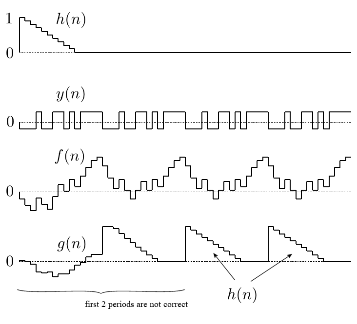
The first two periods of $g(n)$ are corrupted, but from the third period onwards the correct impulse response $h(n)$ is recovered repeatedly (the maximum error is on the order of $2.22\times 10^{-16}$).

Discussion

The first two periods are corrupted because the input to the system is zero before $n=0$, which is inconsistent with the derivation that assumes input periodicity for $n\lt 0$ as well.

Linear convolution of two $N$-sample sequences yields $2N-1$ samples, so over the first two periods the circular-convolution identity does not hold and a transient appears.

For this reason, when averaging, the first two periods (i.e. the first $2N$ samples) must be excluded.

Summary

Starting from a binary MLS $m(n)\in\{0,1\}$, we adjusted the gain and offset to obtain a binary periodic signal whose magnitude spectrum is unity at every frequency,

$$ y(n) = \frac{2}{\sqrt{N+1}}\,m(n)+ \frac{1-\sqrt{N+1}}{N} $$

fed it to the system under test, and convolved the output with one period of the time-reversed signal,

$$ y_-(n) = \left\{ \begin{array}{ll} y(-n), & 0\leq n\lt N \\ 0, & \text{otherwise} \end{array} \right. $$

showing that the impulse response of the system is recovered repeatedly with period $N$. A numerical experiment confirmed the derivation.

Remarks

Because the impulse response was short and $N$ small, an FIR was used for the $y_-(n)$ convolution. For long impulse responses an FFT-based convolution is preferable.

For clarity the derivation kept the magnitude spectrum of $y(n)$ at unity, but the amplitude of $y(n)$ shrinks as $N$ grows. In practice one should multiply $y(n)$ by a gain $A\gt 1$ within the linearity range of the measurement chain and the system under test, and then divide either $y_-(n)$ or the convolution result by $A$ to compensate.

References

Borish, J. and Angell, J.B., "An Efficient Algorithm for Measuring the Impulse Response Using Pseudorandom Noise," J. Audio Eng. Soc., Vol. 31, No. 7/8, pp. 478–488, August 1983.
Kaneda, Y., "An Experimental Study on Errors in Impulse Response Measurement Using an M-sequence," J. Acoust. Soc. Jpn., Vol. 52, No. 10, pp. 752–759, 1996. (in Japanese)
Kashiwagi, H., M-sequences and Their Applications, Shokodo, p. 23. (in Japanese)
Maximum length sequence — Wikipedia

FAQ

What is an MLS?

MLS stands for Maximum Length Sequence, a class of pseudorandom binary sequences. It is generated by a linear feedback shift register and has a periodic autocorrelation that is essentially a unit pulse. This near-impulsive autocorrelation is the property exploited for impulse response measurement.

Why convolve with the time-reversed signal?

If a periodic signal has unit magnitude spectrum at every frequency, then the circular convolution of the signal with its time-reversed copy is the unit pulse $\delta(n)$. This identity lets us recover the impulse response by a single convolution of the system's output with the time-reversed signal.

Why are the first two periods corrupted?

The derivation assumes the input is periodic for all time, but in a real measurement the input is zero before $n=0$. The convolution of two $N$-sample sequences yields $2N-1$ samples, so the first two periods do not satisfy the circular-convolution identity and a transient appears. When averaging, discard the first two periods (i.e. the first $2N$ samples).